library(reticulate)## Warning: package 'reticulate' was built under R version 3.5.2Random Walk Examples in Python
import numpy as np
import matplotlib.pyplot as plt
plt.rc('figure', figsize=(10, 6))
import seaborn as sns
import pandas as pd
np.random.seed(12345)
nwalks = 5000
nsteps = 1000
draws = np.random.randint(0, 2, size=(nwalks, nsteps)) # 0 or 1
steps = np.where(draws > 0, 1, -1)
walks = steps.cumsum(1)
walksarray([[ 1, 0, -1, ..., -6, -7, -6],
[ 1, 0, 1, ..., 46, 45, 46],
[ -1, -2, -3, ..., -46, -47, -48],
...,
[ -1, 0, -1, ..., 0, 1, 0],
[ 1, 0, 1, ..., 104, 105, 104],
[ 1, 2, 3, ..., 14, 15, 16]], dtype=int32)walks.shape(5000, 1000)hits30 = (np.abs(walks) >= 30).any(1)
hits30
hits30.sum() # Number that hit 30 or -303352crossing_times = (np.abs(walks[hits30]) >= 30).argmax(1)
crossing_times.mean()502.1700477326969steps = np.random.normal(loc=0, scale=0.25,
size=(nwalks, nsteps))steps.shape(5000, 1000)plt.figure()
plt.plot(walks[0]);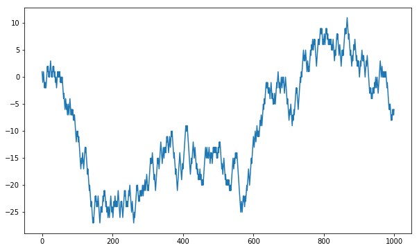
png1
df = pd.DataFrame(walks.T); df.head()| 0 | 1 | 2 | 3 | 4 | 5 | 6 | 7 | 8 | 9 | … | 4990 | 4991 | 4992 | 4993 | 4994 | 4995 | 4996 | 4997 | 4998 | 4999 | |
|---|---|---|---|---|---|---|---|---|---|---|---|---|---|---|---|---|---|---|---|---|---|
| 0 | 1 | 1 | -1 | -1 | 1 | 1 | 1 | -1 | -1 | -1 | … | 1 | 1 | 1 | 1 | 1 | -1 | -1 | -1 | 1 | 1 |
| 1 | 0 | 0 | -2 | 0 | 2 | 0 | 2 | 0 | 0 | 0 | … | 0 | 0 | 2 | 2 | 0 | -2 | 0 | 0 | 0 | 2 |
| 2 | -1 | 1 | -3 | 1 | 3 | -1 | 1 | 1 | 1 | 1 | … | -1 | -1 | 3 | 1 | 1 | -1 | -1 | -1 | 1 | 3 |
| 3 | 0 | 0 | -4 | 0 | 4 | -2 | 2 | 0 | 0 | 0 | … | 0 | 0 | 4 | 2 | 0 | 0 | 0 | -2 | 0 | 4 |
| 4 | 1 | 1 | -3 | -1 | 5 | -3 | 1 | -1 | -1 | -1 | … | -1 | -1 | 5 | 1 | -1 | 1 | 1 | -3 | 1 | 5 |
5 rows × 5000 columns
plt.figure()
plt.plot(df[0]);df.shape(5000, 1000)
test = df.iloc[:, :100]test.reset_index(level=0, inplace=True); test.head()| index | 0 | 1 | 2 | 3 | 4 | 5 | 6 | 7 | 8 | … | 90 | 91 | 92 | 93 | 94 | 95 | 96 | 97 | 98 | 99 | |
|---|---|---|---|---|---|---|---|---|---|---|---|---|---|---|---|---|---|---|---|---|---|
| 0 | 0 | 1 | 1 | -1 | -1 | 1 | 1 | 1 | -1 | -1 | … | 1 | -1 | -1 | 1 | 1 | 1 | 1 | -1 | -1 | 1 |
| 1 | 1 | 0 | 0 | -2 | 0 | 2 | 0 | 2 | 0 | 0 | … | 0 | -2 | 0 | 0 | 0 | 0 | 0 | -2 | -2 | 2 |
| 2 | 2 | -1 | 1 | -3 | 1 | 3 | -1 | 1 | 1 | 1 | … | -1 | -3 | 1 | -1 | 1 | 1 | -1 | -1 | -1 | 1 |
| 3 | 3 | 0 | 0 | -4 | 0 | 4 | -2 | 2 | 0 | 0 | … | -2 | -2 | 0 | -2 | 2 | 0 | 0 | -2 | -2 | 2 |
| 4 | 4 | 1 | 1 | -3 | -1 | 5 | -3 | 1 | -1 | -1 | … | -3 | -1 | 1 | -1 | 3 | -1 | 1 | -1 | -1 | 3 |
5 rows × 101 columns
test2 = pd.melt(test, id_vars= ['index'])test2['variable'] = test2['variable'].astype('category')sns.lineplot(x = 'index', y= 'value', hue= 'variable', data = test2, legend = False, palette = "Blues");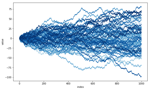
png2
Histograms
test2[test2.variable == 999]| index | variable | value |
|---|
sns.distplot(test2[test2['index'] == 999].value);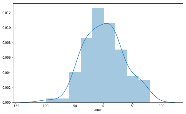
png3